Professor Sir John Enderby FRS (1931-2021): a personal reflection

Shortly before I retired fully from my three decades as an academic at The University of Kent I wrote a short series of blog posts on aspects of my career (starting here). They were drafted in a bit of a hurry in response to a request from one of my colleagues – who was, it transpired, already contemplating a ‘retirement conference’ in my honour and wanted a little biographical material; they were far from exhaustive. Within that handful of posts there is mention of the person who kick-started my career in science in the mid-1970s and who influenced it from time to time for the next thirty five years or so …

When I first came across John Enderby he was ‘Professor Enderby’ and the head of the Department of Physics at the University of Leicester, where I was an undergraduate student. It was years later that he became a Fellow of the Royal Society and was subsequently knighted. Sadly, John died at the beginning of August in 2021; he was 90 years old. Only now, a year later and after the worst of the COVID-related restrictions and fears are in the past, was it practicable to hold a meeting to celebrate his considerable contributions to science. As one of the few people still around who had worked with him during his time at Leicester (and for whom the organisers had contact details) I was asked to contribute to the short talks planned for the first day of the celebratory meeting. It was an honour to accept the invitation. This blog post is, in essence, the distillate of my talk on September 5th at ‘Understanding the Structure of Liquids: Celebrating John Enderby’s Scientific Legacy’ at The University of Bristol.

Family members, friends and former colleagues as photographed at the end of the meeting’s first day by Adrian Barnes. (Should you wish to know, when this was taken I happened to be sitting third row back, second from the right; the image shown below is of the period I was speaking about in my talk.)

An immediate difficulty faced when putting together my slides arose from the lack of contemporary images: the key events took place well before the advent of digital photography or scanners. Photographs were something of a rarity, doubly so in the case of colour. Add to that the fact that I’d been ruthless in clearing out my office as I approached retirement ... I did however find a scanned copy of the above image, taken at a Research Council Graduate School held at Leicester in 1977. John is sitting front left and a very young me stands centre-rear. There are so many distinguished scientists of the time shown in this image, and quite a few early-career people who went on to build amazing careers of their own. (When I first located this image, I confess that one of my initial reactions was to lament the lack of diversity – a situation too often ignored at the time I regret to say.)

In truth, I can’t say I remember anything specific of John until the end of my second year as a naïve BSc Physics student*. I had requested a final year research project in the area of Solid State Physics – an area that had increasingly fascinated me during that year, probably due to some inspirational lecturers – but I honestly couldn’t recount my decision-making process now (even to myself). My project partner and I found ourselves tasked with the study of manganese chloride aqueous salt solutions using Electron Spin Resonance, a technique traditionally rooted within the realm of Chemistry. Could this really be a suitable project in Physics? Our project supervisor was to be none other than Professor Enderby, which was a scary prospect. (I discovered years later that the project’s inception owed much to a conversation that John had had with his research associate George Neilson, whose background was in Chemistry.) This was my first proper exposure to what would eventually shape my own research interests across four decades: the belief that so much of interest lies at the interface between our traditional subject disciplines. For that alone I owe John a huge debt of thanks.

Central to the images above is a monochrome image of the ESR spectrometer we used for our allocated final year research project. It was taken by the departmental technician who acted as official photographer. I was given a copy, as was my project partner, which I annotated by hand and included in my project report – the front cover of which is reproduced on the left. The report itself was typed using a fairly basic typewriter; the equations were inserted by hand as were all graphs, diagrams and tables. I generated a carbon copy for myself; there were no photocopiers in the department. Very few people possessed an electronic calculator at the time, which were still fairly primitive back then – and prohibitively expensive, so calculations were undertaken using logarithms and slide rules.

Unbelievably to us at the time, my project partner and I were invited to a party at John Enderby’s house to celebrate his research group’s success in winning their first truly substantial research grant from what was then the UK Science Research Council. Being made to feel welcome – a part of the team despite our particularly junior status – had a great impact; it afforded one of the many lessons I have sought never to forget. However, there were things to learn from the day-to-day as well. For instance, John’s habit of wandering through the labs. most days, coffee cup in hand, is one deceptively simple example. He’d engage anyone and everyone in conversation about what they were doing; keeping himself abreast of developments of course but, in the process, bolstering the confidence of undergraduate and early-career researchers alike … whilst also keeping them on their toes. With my time as an undergraduate student coming to a close I began the process of sorting out what my next step might be. I had obtained a place on a PGCE course, so secondary school teaching was one attractive option. However, despite enduring feelings of inadequacy, my ambitions were focused on the desire to dive into research. Thus, despite fascinating offers in the areas of ionospheric physics and geophysics, it took me relatively little time to accept John’s offer to join his group as a PhD student.

John’s own 1963 PhD thesis was entitled ‘Some electrical properties of liquid metals’ – my own, submitted sixteen years later wasn’t that dissimilar, although the theoretical landscape had altered considerably in the intervening period. The computational equipment available had progressed a great deal by the time my PhD project came to an end, but the project itself was conducted on a shoestring budget.

"Liquid metals" implies high temperatures – up to about 1750°C in my case – but without much of a budget everything had to be built by hand. Simple angle-iron frames held furnace bricks stacked within an asbestos box (- yes: I had to cut and drill such sheets, the work being done outdoors and using water to suppress dust; different times). The furnaces were lowered/raised using simple screw jacks and the basic vacuum system included copper tubing soldered together by me; I also did all the glass-blowing and the machining of many other components. The colour inset is one of my wife’s still life paintings: a jar like this was used as my primary calibration cell – the whole project rested upon its use!

As it turned out, after a period of study leave in the USA, John left Leicester for a post in Bristol only a year after my PhD began so I never did benefit from his continued day-to-day supervision. One of his Leicester colleagues, Alan Howe, bravely took me on and became my key early-career mentor in John’s stead. John and I stayed in touch however and met on innumerable occasions through the years. This included the period of his tenure as Physical Secretary and Vice-President for The Royal Society, during which time I recall being treated to an excellent meal at the Army & Navy Club so that he could debrief me on my department’s performance in the recent Research Assessment Exercise. I’ve lost count of the number of supportive references etc. he wrote for me, and I have cause to be particularly grateful for his gentle nudges into what became an extensive involvement with the UK Research Councils (see here).

During the first couple of years after the move to Bristol in 1976 John would visit his old department at Leicester often. On just such a visit he wandered into my small lab. for a chat. I wasn’t there, so he had to make do with my latest written log entries. At this point I ought to point out that John was incredibly enthusiastic when ostensibly exciting results emerged, but occasionally this enthusiasm misfired. In the longer term it was never a problem: as the saying goes, first attributed to Nobel Laureate Linus Pauling, “The best way to have a good idea is to have lots of ideas and throw away the bad ones.” John was a master of this approach, which I heartily applaud, but in the short term there are risks. He thought that my data on the resistivity of liquid palladium-silver alloys might represent the first evidence for ‘paramagnons’ in a liquid metal and he duly shared this idea widely. It didn’t, as I demonstrated through further measurement in the months that followed. No long-term harm was done; John was an excellent scientist: when I had generated more reliable data we simply moved on – that’s how science works.

The above are scanned copies of my PhD laboratory logbook pages, the graph on the left and the lower insert being the ones John saw during his unannounced flying visit. It would have been tempting to take this unexpected ‘spike’ in the graph at 33% Ag at face value. However, scientific scepticism – major claims need major evidence – and the desire for both explanation and reproducibility drove me to track down the origin of the feature. My ‘family tree’ of samples (central panel) showed that the ‘paramagnon-like’ feature was evidently associated with a single sample that had been contaminated by the tungsten electrodes I used. This sample, in its turn, contaminated subsequent samples made from it. Given my vanishingly small budget, I had to wait six months before I could buy fresh samples of high purity palladium and silver in order to measure this region of composition again. The graph on the right, although still fascinating in the context of the theories of the time, clearly shows that John’s paramagnons were, sadly, a will-o'-the-wisp.

There were rather few ways in which I could honour John’s scientific contributions, but in 2006 I nominated him for an honorary doctorate at my own university (Kent at Canterbury) which he was able to receive during a formal university degree ceremony. In 2014 I wrote a two-page article in the monthly magazine ‘Laboratory News’ in a short series on heroes of British science – it gave me my penultimate opportunity to pay tribute.

I hope I possess sufficient wisdom to choose to learn from others: to learn what works and what ought to be avoided. I learnt a great deal from John. Indeed, from my days as an undergraduate student, through various transitory research posts and to my thirty years as an academic with my own thoroughly interdisciplinary research team, John remained a person to learn from. I am thankful for the privilege of having known him.

* I had applied for a Joint Honours degree in Physics & Chemistry, but due to an ‘administrative oversight’ I arrived at Leicester to find myself registered for their BSc Physics programme. Lacking the self-confidence to anything other, I simply ‘went with the flow’. I have used the term serendipity often in relation to my career: this apparently random event is perhaps an early example.

A plate from the past: SGT and me

 

I follow many scientists and science-centred organisations on Twitter. In fact, they dominate the list of accounts I follow – which is hardly surprising given my interests. One of these is the Institute of Materials, Minerals & Mining and the other, which is closer to home in terms of my own scientific career in materials research, is the Society of Glass Technology They recently surprised me …

The COVID-delayed sixteenth conference on the Physics of Non-Crystalline Materials was held at the university I worked at before retiring more than seven years ago (see here for details of the current incarnation of my old department). I put something up on Twitter about how strange it felt to have a meeting running for week at my old stomping ground given that, a decade ago, I would have expected to participate. The SGT account holder, who I’ve known for a long time, replied saying that I ought to pop in to say hello as they had something to give me from several years back. How could I resist …

It turned out that they had commissioned a commemorative plate to mark the fact that I delivered the 2015 Mellor Memorial Lecture – the SGT and IoM3 share the hosting of this memorial lecture, and it was the turn of the SGT that year as part of its annual meeting, ‘Glass Reflections’ (here, this is an old link – pre-https days – so your browser may warn you that it’s not secure). I was honoured to be asked. Although I tried hard to prepare properly, I confess that I wasn’t pleased with my performance at the time; I’m almost never pleased with my performance. I was a little taken aback to have all this effort made to honour the event – and completely delighted.

David Moore presenting me with the plate (image taken by Christine Brown). The plate's inscription reads: Presented to Prof Bob Newport by the Ceramics Society - IoM3; 55th Mellor Memorial Lecture 'Glass: out of History and Art and into Tissue Regeneration'; 8th September 2015. The backdrop is a 2018 painting by Heather Gulliver showing an African Coral Tree; it hangs in the PNCS16 conference venue at the University of Kent.

Here’s a little background for you, taken in part from the IoM3’s web site: Joseph Mellor FRS (1869-1938) was a pioneering ceramist and heavily involved in the work of the Ceramic Society (which became the IoM3). He wrote several books including ‘Modern Inorganic Chemistry’. He was elected fellow of the Royal Society in 1927 – no mean feat.

In 2016, in their centenary year, the SGT elected me a Fellow of the Society – an honour I continue to treasure, but have only a certificate in commemoration (see here, second half). That will do nicely.

♪ The Sun has got its spots on … ♫

It has been a whole year since I last posted. I’m sure that this is in part one of many diverse legacies of SARS-COV2, but it’s also related to the fact that my primary focus for the blog was always to reflect on living life as a scientist.* I have in the meantime continued to write about topics in science elsewhere: using my u3a local branch’s social media group example. However, the point is that I intended only to write on this blog as and when my week involved me in rolling up my metaphorical scientists’ sleeves and getting directly involved. You can perhaps see where this is headed …

Last week I visited Year 5 of The Churchill School; one of the two classes is taught by my talented daughter-in-law, and it was she who invited me. I’ve been to the school many times before, but less often as a visiting scientist (e.g. here). I freely confess that school classrooms unnerve me. I (mostly) loved school when I was part of the whole thing as a child and I have the deepest of respect for excellent teachers like my daughter-in-law. However, nowadays, the thought of standing in front of a class of children – let alone two 30+ classes combined – with the aim of leading them into some new knowledge and understanding renders me a little weak at the knees. It was truly lovely, then, to get a warm welcome by the four staff members involved – but it was the eagerness of the 9/10 year-olds that completely blew me away.

I turned up while they were still in a school assembly so that I could get everything set up in peace. I had brought with me my newly acquired second-hand 72 mm refractor, the lightest of my two equatorial mounts and a tray of bits and pieces which included a homemade solar filter. The neutral filter material, which removes 99.999% of the incident light, is of the highest standard, but I can’t say the same thing about the cardboard and duct tape assembly that holds it in place in front of the telescope’s objective lens. In order for the equatorial mount’s tiny battery-driven motors to keep the telescope pointing towards the Sun over time, it has to be tilted to the correct latitude, levelled and compass-aligned. The telescope itself also needs to be balanced (both front to back and side to side). Once the Sun had been located and its image focused I have to say that I was more than relieved to see several sunspot clusters clearly visible; passing clouds were, as ever, less predictable. (By the way, the images taken at the school were carefully checked by them before they were released for my use; faces have been covered/blurred as necessary.)

I was given a generous introduction inside the school before we all trooped out to the school’s expansive playing field and the children sat in a semi-circle on the summer-dry grass. I kept my own introduction to the telescope very simple; no-one needed to know about focal lengths and lenses in order to observe the Sun. What did need to be shared at the outset though was the standard but ever-vital warning not to look directly at the Sun for fear of damaging the eyes. In this instance it was important to go much further, making the point that looking at the Sun through binoculars or a telescope is likely to cause blindness without the appropriate safety measures in place. You also have now been warned 😉

I had given them a rough idea where the sunspot clusters were by describing the Sun’s disk as a clock face: two and eight o’clock got them to the most obvious, although it was a busy day on the Sun and there was a lot to choose from. This is an image captured by a talented amateur astronomer, Roger Hyman ( find him here or here) on that same day; the image is used with his permission. The orientation isn’t exactly as we saw it – the angle of the camera he was using and other factors will affect that, but it’s close enough. All clusters of sunspots are given a unique identifying number and on Friday 15th July 2022 they were, beginning at the 2:30 position and moving clockwise: 3057, 3056, 3055 and 3053 (see here).

In between the slowly drifting clouds, everyone got a chance to look through the telescope – even the adults. All but a handful said they’d seen the sunspots: some after a bit of coaching in terms of how to use an eyepiece. It took a while, and given the need for a lot of patience they did astonishingly well.

Every time a cloud came over we used it as an opportunity for questions, which came thick and fast. Indeed, the flow of questions continued when everyone had had the opportunity to take a peek and we had moved back inside the building. These were exceptionally wide-ranging, and varied from the scientifically and philosophically challenging to the more speculative ‘what if’ (the Sun disappeared, you went into a black hole, …) and ‘would you’ (like to go into space, live on Mars, …) type of question. All of them deserved to be taken seriously and given the best response I could muster. I can only say that I was genuinely impressed; it was uplifting to see so much evidence of the potential on display within that classroom. A few of them were obviously highly clued up, and several made a point of telling me that they wanted to be a scientist. Perhaps what I should have said in response, but for some reason didn’t, is that in a sense they already were – just as much as I was at their age.

I was at the school for almost 2½ hours in total, although it felt far briefer than that.

I promised this blog post in order to provide a reminder of what we did, and to offer a little information in a more coherent way than I fear I managed on the day. Perhaps one might start by saying that sunspots are associated with a localised increase in the Sun’s magnetic field. They appear darker than their surroundings simply because they are a little cooler, with their central region (the umbra) at about 3000-4000ºC compared to the average of 6000ºC. Their sizes vary a great deal, with the largest being several times the diameter of the Earth. (If you are able to see the above image of the Sun on a reasonably large screen then you might notice the small blue dot I inserted to the left hand side: that is approximately the size of the Earth on the same scale.) Sunspots can last for days, but eventually disappear. The number of sunspots visible at any one time varies over the eleven years of the solar activity cycle; we’ll be at the next maximum in this cycle in 2024. You can find lots more information here, here and here; a recent BBC ‘Sky at Night’ programme covered some of this ground also.

Perhaps a fitting way to close this post would be to offer a couple of suggestions for useful astronomy apps and to share a small number of my own images. The first app I downloaded when picking up after retiring the hobby of my youth (from Android Play Store) was ‘Sky Map’, which I still use as a simple interactive guide to the sky; for a little more sophistication one might go for ‘Stellarium’. The choice is yours. In addition, and especially if you want to pursue this further, I’d recommend joining your nearest amateur astronomy group. Unfortunately, the one I’m in – Ashford Amateur Astronomy Society – is an hour’s drive from my home; maybe there’s one closer to where you live.

The above were taken at different dates, through different telescopes and with different cameras. The result is that we have a fairly recent image of the whole disc of the Sun together with a more highly magnified image of one part of the solar disc, and a close-up of two particular sunspot clusters taken in 2021 which bring out a bit more detail in terms of their structure. You’ll notice that each sunspot comprises a dark central region (the umbra) and a somewhat bright outer region (the penumbra); as you might anticipate, the penumbra has a temperature which is intermediate between the umbra’s and the Sun’s average surface temperature.

Happy observing.


* I retired from my paid employment as an academic and multidisciplinary materials research team leader about seven years ago, but I’m still a scientist – just as I was as far back into childhood as I can remember; I’ve covered this ground in earlier posts (e.g. here).

Pictures of home

Our home, Earth, is a rare and peculiarly beautiful planet: a bright sphere effortlessly pirouetting through the black. In reality, it’s constrained within a routine choreographed by gravity and conducted by its home star, the Sun. Moreover, it doesn’t dance through space-time alone but with a partner in the form of the Moon – the relationship between them as unusual as the planet itself. Even the Sun is unusual within its peers. Our home planet is at one and the same time just like all the other countless planets in orbit around trillions of stars and yet, as far as we know, so unusual that we might even be tempted to call it unique. The mere fact of our presence on its surface, beings able to ask the searching questions we do, marks it out as special.

I have written about the Earth before (here), and during lockdown I recorded a talk on the subject (find it here). I’ve no intention of revisiting this material in detail – there would be no point – but I am going to celebrate the Earth in another way by sharing with you some of the images captured during my lifetime that have had a particular impact on me in one way or another. (I note in passing that the entirety of humankind’s rocket-based space exploration endeavours thus far have occurred during my life.) Given the thousands of beautiful, informative and sometimes shocking pictures taken from orbit – through the windows and lenses on the International Space Station for example – one might become a little blasé, or perhaps overwhelmed, by the choice on offer. Fear not, I am side-stepping them all; rather than study these ‘close-ups’ I want to share with you my enjoyment of the long-shots: the images captured from afar which reveal the whole Earth in its role as a rocky, water-rich ‘Goldilocks’ planet within our solar system. I might allow the Moon a look-in as well …

Although not the first picture of our home chronologically speaking, my all-time favourite image is arguably one of the poorest in terms of photographic quality: the so-called ‘Pale Blue Dot’ captured by Voyager 1. It was taken just before its cameras were turned off to conserve power as it headed towards the very farthest reaches of the Sun’s dominance and thence into interstellar space. Voyagers 1 and 2 were launched separately during the summer of 1977 (see here for more information; I was in my mid-twenties at the time!). Both were designed and built to provide the first close-up look at Jupiter and Saturn; Voyager 2 would in addition fly on to Neptune and Uranus, the outermost planets in the Solar System. The mission was to last five years … it’s still in progress four decades later, adding new science to an already astonishing portfolio. That fact alone sets the Voyagers apart in my imagination, but there’s so much more: to have designed a mission of such complexity on what was, relatively speaking, a modest budget and with the very basic electronic computers available at the time remains a triumph of scientific and technological endeavour. I still keep in touch with the mission’s progress via the Voyager Twitter feed.

On February 14th 1990, Voyager 1 was instructed to turn its camera and photograph the planets of our solar system whilst it was still just about possible. It was by then six billion kilometres from Earth. At this distance Earth appeared so small and so close to the position of the Sun that it was barely possible to capture anything at all. As it was, Earth represents only about 1/8th of a pixel and sits within optical artefacts – the streaks of light – caused by the much brighter sunlight entering the camera via its colour filters. The Sun itself is just out of shot. Venus was similarly difficult to capture; neither Mercury nor Mars could be imaged at all because of their positions with respect to the Sun. (I've added arrows to help you see the tiny bright dot that is Earth.)

‘The Pale Blue Dot’, in spite of its limitations, easily remains at the top of my list of the all-time-great pictures of our home planet. However, an image captured much earlier in the mission (far left) hovers somewhere nearby in terms of its ability to captivate my mind, my imagination. Only a couple of weeks after its launch, Voyager 1 took this picture of the crescent Earth and Moon from a distance of 11.7 million kilometres, and in the process illustrated the mission’s later potential. This was the very first time that the Earth and Moon had been captured in a single image (- the Moon is upper left; it's relatively dull compared to the bright Earth). Many analogous pictures have emerged over the years, each special in their own way. In the centre is a 2017 greyscale picture captured by the ORIRIS-Rex probe on its way to rendezvous with an asteroid. (Because the Earth is so much brighter than the Moon, the image has been processed such that the Moon’s brightness is enhanced by a factor of three.) In 2010 the Messenger probe, sent to study the solar system’s innermost planet, Mercury, looked back out and away from the Sun to capture the view of the Earth⸱⸱⸱Moon duo shown on the right. When viewed from the vicinity of Mercury, both the Earth and the Moon will always appear as bright full discs – no elegant crescents from this perspective. There are so many other broadly similar Earth⸱⸱⸱Moon shots of this type available online; I’ve pruned my selection heavily for this blog and in the process cut superb images such as those shown here and here.

If the ‘Pale Blue Dot’ tops my personal list of iconic pictures of home, then a very close-run second place must go to one of the staggeringly beautiful images captured by the Cassini probe during its extended sojourn at Saturn. This one (top) was taken in 2013 with Saturn backlit – in other words we’re looking at its night-time face with sunlight scattering through the ring system and outer atmosphere. A lower right segment of the wide-angle full image, shown lower left, reveals the Earth peeping out from behind the rings (there’s an arrow to help you locate it; Earth is about 1.4 billion kilometres away and at that distance each pixel of Cassini’s camera covers almost 9000 km of the Earth’s surface). Enlarged further in the lower right panel, we can easily discern the Earth⸱⸱⸱Moon duo. For sheer majestic beauty it would be hard to beat such a picture of home. In passing, note the apparent absence of stars in these pictures. The reason for this is simply that they are too faint to show up in an image focused on such a bright target.

Moving a little closer to Earth again, I’ll share with you a picture of home that also captivated me: an image taken from the surface of Mars by the Curiosity rover in 2014 (here). It’s nothing special in terms of photographic quality, but it’s reminiscent of the sort of photo one could take of Venus, say, from here: from the surface of one planet, a bright point of light in the evening sky which turns out to be a neighbouring planet. Almost homely. The central panel shows a reprocessed version of the picture with an enlarged inset of the Earth⸱⸱⸱Moon system. Taken at these sorts of distances we can be sure that the relative sizes of the Earth and its moon are about right; although even here one needs to consider the fact that the Moon and the Earth orbit each other such that their separation in space as viewed through a camera lens may appear to change. (Technically, they both rotate about their Barycentre – their centre-of-mass; see my blog post or YouTube video on the Earth for an explanation.) For pictures captured closer to home, like those shown in the Voyager/Osiris/Messenger images above, one needs to be even more careful since the apparent relative diameters may be heavily influenced by their respective distance from the camera. On the right hand side above I have inserted an image I captured on my smartphone of the crescent Moon and crescent Venus: Venus is, in reality, far larger than the Moon – but it is of course much further away from my phone than is the Moon, even if it does appear in the same part of the night sky above my garden.

An interesting thought poses itself in the context of these images of Earth from the Martian surface: how would one observe Earth through a telescope in the way we might observe Mars? The same considerations pertain for Earth observation from the lunar surface. One would be unable to look directly through a telescope eyepiece of course since there would be a spacesuit visor in the way. For a more considered exploration of this ‘thought experiment’ I recommend an article in the ‘Sky at Night’ magazine, here.

I have followed the development of space exploration from about the age of six – I remember Sputnik and Telstar, the first animals to travel to space (and die there) and the start of crewed missions – and was in my mid-teens when the first astronauts left their footprints on the Moon. Although the video images beamed back to our monochrome and distinctly low-resolution TV screens were epoch-defining, they were nothing to write home about in terms of image quality. However, the images taken by crew members …

The Apollo 8 mission involved using the Earth’s and the Moon’s gravitational field in order to do a loop around the Moon before coasting back to Earth; the crew practiced most of the manoeuvres necessary for a Moon landing without that final all-important stage. In the process, they captured a series of pictures which have become truly memorable. Later missions, through to Apollo 17, added to this collection and/or improved picture quality. Two of the more iconic pictures of home are shown above: ‘Earthrise’ and ‘The Blue Marble’. The latter is fairly self-explanatory, although it’s worth pointing out that the inclusion of a view of Antarctica was a novelty at this stage of the game. ‘Earthrise’ does need some discussion though. The fact of the matter is that Earth never actually rises: the Moon is tidally locked to the Earth, meaning that the same lunar face is always pointing toward us – how could we talk of the far side of the Moon otherwise. So, if one face is permanently facing Earth then it follows that the Earth is always visible above the horizon from half the lunar surface and always invisible from the other half: there is neither rising nor setting. (Just to amuse yourself, take a look at this gif which shows the Moon ‘photo-bombing’ Earth – what we can see here is the far side of the lunar surface, the side we can never see directly from our planet.) However, as the Apollo crew were orbiting the Moon it would appear from their perspective that the Earth rose and set each time they went around. The image on the far right is the actual orientation as seen from the orbiting command module; only by rotating the picture was it possible to present to us the final evocative picture of home as seen on the left. Unsurprisingly, ‘Earthrise’ became a poster-shot for the growing environmental movement of the day.

I might have stopped at this point had the chair of the Ashford Astronomy Association*, Jason, not reminded me of another series of spine-tinglingly good shots of our home world taken by Apollo mission crew. There exists some excellent video footage of the astronauts’ ascent from the lunar surface to re-join the orbiting command module (see here for example), but some of the stills are truly astonishing. The image above is one such: Moon in the foreground and Earth, home, shown in the distance.

I hope you have enjoyed my little gallery of pictures of home; feel free to share your own.



* I joined this lovely club a few months before ‘lockdown’; we’ve been meeting via Zoom ever since. I’ve had lots of good advice from its more experienced members which has probably saved me countless hours of trial and error when trying my hand at astrophotography, and some pretty decent suggestions for beautiful things to observe.

Conversations: from screen to woodland

Many years ago I discovered the joy of sharing my love of science with non-experts: initially within schools (all the way to Years 4 and 5, e.g. here) and then to lay adult groups. Since retiring I’ve focused primarily on the lovely retired or semi-retired people of the U3A, both in my home town (e.g. here)and more widely e.g. here). I have learnt, and continue to learn, how to communicate science-based topics. Spending more than four decades speaking at meetings and conferences, and three of those teaching physics students, has brought me to the point of being able to perform satisfactorily – yes, teaching is in part a performance art – and to enjoy the process. I’d now miss being able to talk to people about science and being a scientist. All this has taken place against the background of being a social/thinking introvert (see here for an explanation of these terms).

However, woven through those Science Communication activities has been a less conventional thread: invitations to join projects associated with festivals (e.g. here and links therein) and others coming from the arts (e.g. here or here). Each of these latter activities has taken me away from anything I might describe as my comfort zone; they have been ‘scary’ at one level or another, but also immensely rewarding. There have been fewer such opportunities since I retired, which is both understandable and a little sad. In a year of SARS-COV2 lockdown I confess to expecting nothing of the sort to come my way. What a lovely surprise, then, to have had two invitations arrive: it is these two activities – a recorded conversation for a new podcast series using Zoom and a conversation about and within the natural world as part of a broader philosophical project.

Towards the end of June 2020 I had an email from Dan Harding. I am a long-time admirer of his work as Director of Music Performance at my old university and I follow his Twitter stream and music blog assiduously. Exactly as I had done in the context of the U3A, he too had decided that lockdown required of him another new venture: this one would comprise a series of podcast conversations on the theme of creativity within the pandemic. The series title captured the essence of the experiment very well in my opinion: ‘Zoom for Thought’. His email invited me to participate in the first episode. I went through my usual list of reasons why I absolutely couldn’t do this – it’s a long list – but said “Yes” anyway. A conversation with Dan is always a pleasure and this screen-mediated one was no exception, despite its novelty. I came away pleased I had agreed to do it and uplifted by the fresh recognition of so many aspects of creativity that transcended the differences between our respective areas of expertise. There have been many guests since, all more erudite and accomplished in areas I am not, and the podcast is now in its second series: do listen if you have a mind to.

“The first episode features a conversation with Bob Newport, Emeritus Professor of Materials Physics at the University of Kent. In which we talk about finding creative ways of continuing to explore physics at home, engaging listeners during lockdown in both science and music, finding teaching tools within the home and grappling with the exciting unpredictably of a dodgy wifi signal... "I'm an experimental scientist, after all: I should be good at putting odd things together," Having retired from teaching at the University of Kent, Bob now teaches for the University of the Third Age in a series of blog articles and videos. Since lockdown, Dan has been engaging the community of musicians at the university through the Virtual Music Project, creating a series of recordings of music by Vivaldi and Mozart from recordings made in isolation…” Taken from here.

Skip forward to March 2021 and a message from Sarah Dance via Twitter. I first met Sarah many years ago in connection with one of the less conventional science communication avenues mentioned earlier; she works in the arts and creative industries (see here) and has been based in my part of the UK for a couple of decades. She was playing match-maker, and her follow-up email ‘e-introduced’ me to Russell Burdon in the context of his current philosophical artistic project (see here). To paraphrase the project’s website, his art residency seeks to deliver responses to the landscape and its biodiversity and history as he finds inspiration – and this inspiration may be fed from across intellectual disciplines and media types … enter yours truly, stage left, scientist.

Russell and I met a few weeks later on a sunny day and spent almost two hours walking and talking on and around the Crab and Winkle Way https://www.sustrans.org.uk/find-a-route-on-the-national-cycle-network/crab-and-winkle-way/, mostly on pathways through mixed woodland. I say ‘walking’ as though there might have been planned and purposeful progress, but in truth there was a lot of strolling and quite a bit of standing still. The conversation let up only when an unusual butterfly or colourful patch of wild flowers held our gaze for a while. We had some things in common but by no means all, and together with a willingness to be open that admixture led to an unpredictable but wholly positive flow of words in pursuit of understanding. I’m not sure whether my contribution from the perspective of a scientist in retirement will prove useful within Russell’s project but, either way, I’m looking forward to seeing what eventually emerges.

In his novel ‘Till we have Faces’, a re-telling of the classical myth of Cupid and Psyche, C.S. Lewis uses the phrase “words going out to do battle with words”; sometimes words play a far, far more constructive role.

As the 1990’s TV advert told us: “It’s good to talk”.

Castor

This is in a very real way a postscript. My previous post, Mizar, marked something of a turning point in my pursuit of astronomy and then astrophotography. I wrote of a childhood hobby, carried out on a pocket-money budget and before personal computers were dreamt of, now reborn in retirement with a modest, but nevertheless much-improved budget. The evening’s observations that had given rise to that post had seen me reach a place of comfort with telescope, astrocam, software … in fact, the whole kit and caboodle – a place of more confidence than happenstance or happy accident. There remains more to learn than is already learnt, that probably goes without saying given my continuing status as a novice but I have at last passed my ‘driving test’. Thus, with a second clear and still night presenting itself in as many weeks – a rare coincidence this past winter – the temptation to set everything up again and try out my new skills was irresistible.

Gemini: a set of stars at all sorts of distances from the Earth – i.e. not bound to one another in any meaningful sense other than that they all reside in our galaxy, The Milky Way. Gemini is an aphorism, not a constellation. Their brightness and apparent proximity suggested particular shapes to our forebears; this is a much-studied form of ‘pattern-recognition’ (see here for a brief article outlining current thinking on the process.)    (Image created from ‘Stellarium’, a free-to-download computer package allowing one to generate bespoke star maps.)

Serendipity provided me with a ready-made target. The vice chair of the amateur astronomy society I joined shortly before the SARS-COV2 virus appeared in the UK (Steve, see here for details) had recently posted a detailed review of the night sky in spring. Within this was a section on the aphorism Gemini. In particular, it mentioned the constituent star Castor, a binary system much like Mizar in some ways. It has two principal components and a more distant third – each of which is itself a binary, the partners all being too faint and too close to observe directly; so six stars in all, just like Mizar. Six stars, five orbits; all taking place about 51 light years away (see diagram below). This was interesting in a generic sort of way, but the key factor for me was that the two brightest stars orbit each other at a relatively small distance. Indeed, from Earth, their angular separation is only about 6 arcsec*. Thus, I had a pretty good test subject for the claim I made in my post on Mizar: that I could probably fully resolve objects only ~5 arcsec apart. The game was on.

Each of the three paired partners orbiting each other, that’s three; Castor A and Castor B orbiting each other, and then finally AB and the two Castor C partners orbiting each other. Again, highly analogous to the Mizar ‘sextuplet’: a beautifully complex dance to gravity’s tune.

Castor was going to be pretty high in the sky at the times I was planning to observe it so, by keeping the tripod and mount relatively low to the ground, extending the legs only in order to level the mount, the small finder-scope was still easily useable without needing to balance on steps! The image was taken using the red-light torch bought for me by my daughter; it’s a light that doesn’t wreck ones night vision. By contrast, right at the top of the image is one of the nearby street lights that can be quite a nuisance, although less so than external security lights and passing car headlamps. Unfortunately, to get a view of both Polaris (for Polar Alignment of the mount) and of the southern sky for a lot of the interesting stuff, the front of my drive is pretty much my only option. On the positive side, it’s led to several lovely (socially distanced) conversations with passing ‘night owls’. The picture on the right is of my laptop display as I located Castor – the A⸱⸱⸱B stars were immediately visible; I’ve circled the pair. I confess to staring at the screen for a minute or two; in part this was the pleasure of seeing two well-resolved stars, but it was also in growing celebration of the fact that I had at last ‘cracked’ polar alignment – there was only minimal drifting of the stars on the screen.

This is the final stacked image showing Castor A and Castor B (lower right); an enlarged version is inset (upper left). The image represents the best 30% of 5000 40 ms sub-exposures. The two stars (or rather, the two pairs of stars – their respective partners being too faint and close to observe directly) are well-resolved: my system’s estimated resolution would seem to be entirely justified. The labelled figure shown below will clarify this further I hope. Castor A and B orbit each other with a period of about 445 years; their partners, Aa⸱⸱⸱Ab and Ba⸱⸱⸱Bb have orbit times in the region of 9¼ and 3 days respectively.

Given my fixation on the relatively bright near-neighbour Castor A and Castor B pair I confess that I didn’t even look for the more distant Castor C. Given that the pair are classified as cool dwarf stars and have luminosities less than 10% of the Sun’s, and that they eclipse each other as they orbit around their common centre of gravity (their barycentre: see my earlier post here) it hardly seemed worth the search. I was wrong. What I should have done was to collect data at longer exposure times, ignoring the fact that the A and B stars would be over-exposed; nevertheless, by increasing the brightness of the stacked image in my old version of Photoshop it was still just about possible to make out the third component: Castor C. This is shown in the inverted (‘negative’) image below. Caster C orbits the AB system every 14,000 years approximately; the pair of stars making up this faint companion orbit each other in a little under 20 hours!

The labelled and annotated figure above summarises the results of my evening’s observational experiment; the images have been inverted ('negative') in order to show Castor C more clearly.

Facts and figures beyond those offered in the stargazing guide referred to at the opening of this post were taken from two online sources: here and here. Both sites contain a wealth of additional information should you wish to learn more. One additional fact with which to close the post: because the orientation of their orbit is not face-on to the Earth, the angular separation of Castor A and B varies with time: in 1970 it was only 2 arcsec and by 2100 it will reach a maximum of 6.5 arcseconds.

______________________________________________

* From one horizon across the arc of the sky to the opposite horizon is 180º (i.e. half a circle), but a degree is too large a unit for many purposes, so we may divide it into sixty arc minutes (arcmin, sometimes simply ′). The Moon and the Sun both appear to be about 30 arcmin across for example, ½º. Even an arcmin is too large on occasion so we may divide that again into sixty arc seconds (arcsec or ′′). (This extract taken from my previous post, here.)

 

Mizar

My father was part-way through his apprenticeship as a bricklayer when the light escaped from its star and began its journey across space. He had left school in his early-teens, as was the norm for working class kids back then. War in Europe was brewing, and although he didn’t yet know it he’d soon be lying about his age so that he could sign up for the parachute regiment; his apprenticeship would be put on hold for the duration. Skip forward eighty three years to the present day; to be precise, to the tail-end of the day on which the Sun had set on 2020-21’s astronomical winter: the night before the Vernal/Spring Equinox. The sky was clear and there was only a slight breeze: almost perfect for a bit of star-gazing. Within the hour I could be found in my front garden looking back in time, in a manner of speaking, to those late 1930s. My target for the evening was Mizar in The Plough, a part of Ursa Major. Mizar is a binary star system which sits at about 83 light years (ly) from us – in other words, the light which fell into my telescope that evening left the stars’ surface 83 years ago. As it happens, the Mizar binary system is more intriguing than it appears at first sight: it has a few surprises up its metaphorical sleeve.

On the left is Ursa Major – the Great Bear. Technically, we ought to be calling it an asterism rather than a constellation since it has more to do with our innate human tendency to invent patterns where there are none than it does to an objectively fixed shape. Although some of the stars in Ursa Major are at roughly the same distance from us (in the region of 80-85 ly, light years – the distance light travels in eighty years) and have similar trajectories in space, others do not. Thus, in times past and in times yet to come what we might perceive as a bear would have appeared/will appear quite different. Mizar forms a particularly noticeable star within part of the large asterism of Ursa Major – it’s the kink in the prominent arm of what is commonly called The Plough (or Big Dipper, or Saucepan, or …). The images used above are taken from ‘Stellarium’, a free-to-download computer package allowing one to generate bespoke star maps.

My primary goal since beginning to dabble in astrophotography after my retirement has been to gain reasonable images of each of the planets in our solar system; to this I might add a long list of lunar features and a sunspot or two. I’ve made a start (see former posts here and here) but there’s so much more I want to do. Moreover, along the way I’d also like to capture images of a few more distant objects: galaxies, star clusters, nebulae. All this requires that I gain an understanding of what my telescope + astro-camera can achieve and the ways in which I might realise that potential. For instance, the telescope’s focal length and magnification, and the size of the CCD chip in the camera together limit the effective field of view (FoV) available to me and define the resolution achievable. Again, in the post immediately previous to this one I mentioned the need to align the telescope’s mount correctly using the Pole Star (Polaris) so that an object might be accurately tracked across the sky as the Earth rotates beneath. This is a task rendered difficult and uncomfortable, even painful, when one tries to manage it with creaking knees and an inflexible spine – finding a way to mitigate this remains on my ‘to do’ list. (I'm tempted to remark that the designers of the polarscopes on the market have really missed a trick here: building in a mirror or prism to allow the eyepiece to face outward or upward would solve this problem at a stroke.) I also expressed the hope that I could, with my smartphone attached to the telescope, use one of the many sky chart apps as a way of navigating to particular target objects. Thus it was on this particular evening that I decided to do some experiments in order to explore the issues. Given the aim, what follows almost necessary contains a technical element to it; hopefully not too much.

Although I currently see no way around the physical discomfort of the polar alignment process, I did at least achieve some success this time around – and the data to verify that statement. The results weren’t perfect, but I think I understand why. Objects initially centre-screen were therefore still drifting slowly off. Next time. However, by focusing on a star and generating images as a function of the exposure time, one can see when the image ceases to be circular and develops an elongation due to the inaccurate tracking. That is to say, we can ask how long an exposure is possible before there is blurring due to the star’s apparent motion across my laptop screen. Now, for all astrophotography it is necessary to collect a number of individual sub-exposures and then stack the best of them to generate a final image since this allows one to reduce the issues of atmospheric turbulence. For the purposes of this exercise I collected 500-1000 ‘subs’ and typically used the best 30% of them. The results are shown below.

These images show Mizar A and B (see below) with sub-exposures set to 51, 67, 130, 300 and 500 ms (milli-seconds) respectively left to right. The three shortest exposure times generated final images too faint to show up clearly in a blog post and I have therefore artificially altered the brightness. Only at 500 ms (i.e. ½ s) do we see evidence of distortion in both stars. Improved polar alignment will hopefully allow the extended exposure times of a few seconds required for more faint objects. However, even the results shown here are sufficient for the solar system targets I have in mind, and a great deal more besides. (I ought to note that the camera focus, a critical preliminary stage in the overall experiment, was achieved using a Bahtinov mask as discussed in earlier ‘stargazing’ posts.)

The images shown above give us a first insight into the complexity of the Mizar binary system. Now, the binary star that one is supposed to be able to see with the naked eye, but which in practice requires good eyesight and the absence of light polluted skies – or the use of a pair of binoculars – comprises Mizar and the fainter star Alcor. They are at a distance of approximately one lightyear (1 ly) from each other and are therefore only weakly bound together gravitationally; they therefore take several hundred thousand years to orbit each other. It turns out that Mizar and Alcor are themselves both binary stars, and whilst the dwarf star associated with Alcor is too small/dim to be seen directly, the Mizar binary – Mizar A and Mizar B – can be resolved even with my amateur setup. These two stars, one much brighter that the other, orbit each other every 5000 years or so at a very close distance – only about ten times the distance from the Sun to Pluto. It takes about 5½ hours for the Sun’s light to reach Pluto, meaning that the Mizar A⸱⸱⸱B distance is only about 55 lh (light hours; the Earth orbits the Sun at a distance of approximately 8½ light minutes). The stars are all relatively young at about 370 million years; by comparison, the Sun is approximately twelve times as old at 4½ billion years.

The above is an inverted image of the view I captured. (I inverted it simply because it’s easier to see ‘black’ stars against a pale background; the superimposed circles should also help.) Mizar A and B are on the right and Alcor – the principal component to the binary system visible with binoculars – is on the left. The figures shown below will hopefully be easier to follow as I’ve added labels. The image is the result of stacking the best 40% of 1000 individual 75 ms frames, so 30 s in total. I probably ought to have collected more data, but the evening’s experiment was about testing my stargazing equipment rather than achieving polished pictures.

We’re not finished with the complexity of this system yet: both Mizar A and Mizar B have been discovered to be binary stars in their own right (Aa and Ab, Ba and Bb should you have a desire to label them). These pairs have orbital periods as short as three weeks or so. As with Alcor’s partner star, they are not visible using anything other than the most sophisticated equipment. However, it’s still an interesting star system to have examined: not a simple binary pair at all but rather a multi-star system – a sextuplet if you will. I was delighted to have seen three stars within the system although being able to add something of their ‘backstory’ enhances the fun. There are several good descriptions of the system available online, e.g. here, here and here .

We need to cover a few preliminaries before I can tell you what the results reveal. Specifically, we need to understand the measurement scale used to describe the apparent separation of two objects in the sky. From one horizon across the arc of the sky to the opposite horizon is 180º (i.e. half a circle), but a degree is too large a unit for many purposes, so we may divide it into sixty arc minutes (arcmin, sometimes simply ′). The Moon and the Sun both appear to be about 30 arcmin across for example, ½º. Even an arcmin is too large on occasion so we may divide that again into sixty arc seconds (arcsec or ′′). Having got that under our belt, the diagram below shows the results obtained.

The Mizar⸱⸱⸱Alcor separation as seen from the Earth is about 11.8 arcmin. This separation gives me the chance to measure experimentally my telescope+camera’s field-of-view. On this basis I estimate my equipment’s field-of-view – the amount of the sky displayed on my laptop screen – to be 16 x 9 arcmin. This is small; it’s no wonder I have to make mosaics in order to create an image of the Moon. The Mizar A and B pair offered one more useful measurement. When viewed from the Earth they appear separated by 14.4 arcsec; this suggests that I can hope to resolve objects separated by only 4-5 arcsec. I’m quite happy with that.

Dad would have enjoyed reading this post, not because he was into astronomy as such, but nevertheless ...  Only later in my life, when I had watched my children begin to shape their lives, did I more fully realise how important his support had been as I moved inexorably towards a life so different to his own. This included helping me to buy my very first telescope, which I still have. It therefore seems entirely natural to think of him as I reflect on my evening with Mizar.

More pictures of a stargazer

Back in August 2020, whilst those in the UK who were not designated ‘clinically extremely vulnerable’ were enjoying a transitory relaxation of covid-19 lockdown rules, I posted a synopsis of my early attempts at astrophotography (here). This was my celebration of a return in retirement to the hobbies of childhood and teenage: astronomy and the geeky side of photography. I remain moderately pleased with the images I shared then and offer now, even though they bear no comparison to those readily available online from professionals and experienced amateurs alike; the essential point is that they are my images. The targets were tracked down by me (without the benefit of an automated navigation system, often referred to as a ‘GoTo’ system) using a telescope I had set up; the images were captured to my laptop’s hard-drive and the data processed using the desktop in my study. It’s personal. Having said that, most of the targets were fairly easy to find and I used only the necessary basic levels of data processing software. This seems like an opportune moment to record and reflect upon my progress … such as it is, given the dearth of suitable conditions for observing during this past year. The fact of the matter is that I not only need a clear sky but also the near-absence of wind in order to get anywhere at all. Even when both criteria are ostensibly satisfied there may be too much turbulence in the upper atmosphere to achieve anything much. Nevertheless, fun has been had and I continue to take baby steps forwards.

New images.

Top row left to right: Tycho, an impact crater near the Moon’s South pole; Mare Nectaris, the Sea of Nectar lava plain; Clavius, an impact crater (note the bright ‘rays’ coming from it: these contain reflective glassy materials).

Middle row: the Mizar A-B binary star system in The Plough; Uranus (image expanded).

Bottom row: M42, the star-forming nebula in Orion (my second attempt, the first being in my previous post); Betelgeuse, a red giant star in the same constellation (image expanded). The green glow in M42 comes from the oxygen atoms in the cloud glowing as they are bombarded by light from those four bright central stars – it’s the same physical process that gives us the aurora on Earth.

The topmost video is of a single star imaged onto my laptop screen; the evening had been perfectly still when I was setting up then a breeze started: only 7 mph, but with modest gusts - the results are self-evident. Even on a still night, upper-atmosphere turbulence can distort the image in the way shown in the lower image of the Moon.

One of the purchases I made has eased the fraught but absolutely essential process of achieving a precise telescope focus. As purchased, my telescope had a manual rack-and-pinion focusing wheel; classic. I described the frustrations of its use in my earlier post. Thus, when I saw in a sale a motorized drive I could retrofit to the focus mechanism I snapped it up. Now I can alter the focus without setting up vibrations in the telescope and needing to wait for everything to settle down between each adjustment as I hone in on the perfect setting. Moreover, this also made it practicable to use a software tool in conjunction with my Bahtinov mask – also mentioned in the previous post – which provides a real-time quantitative estimate of focus quality.

A frightening level of force was required in order to twist off the original wheel (identical to the remaining wheel at the top of the image; it was glued onto the threaded shaft).

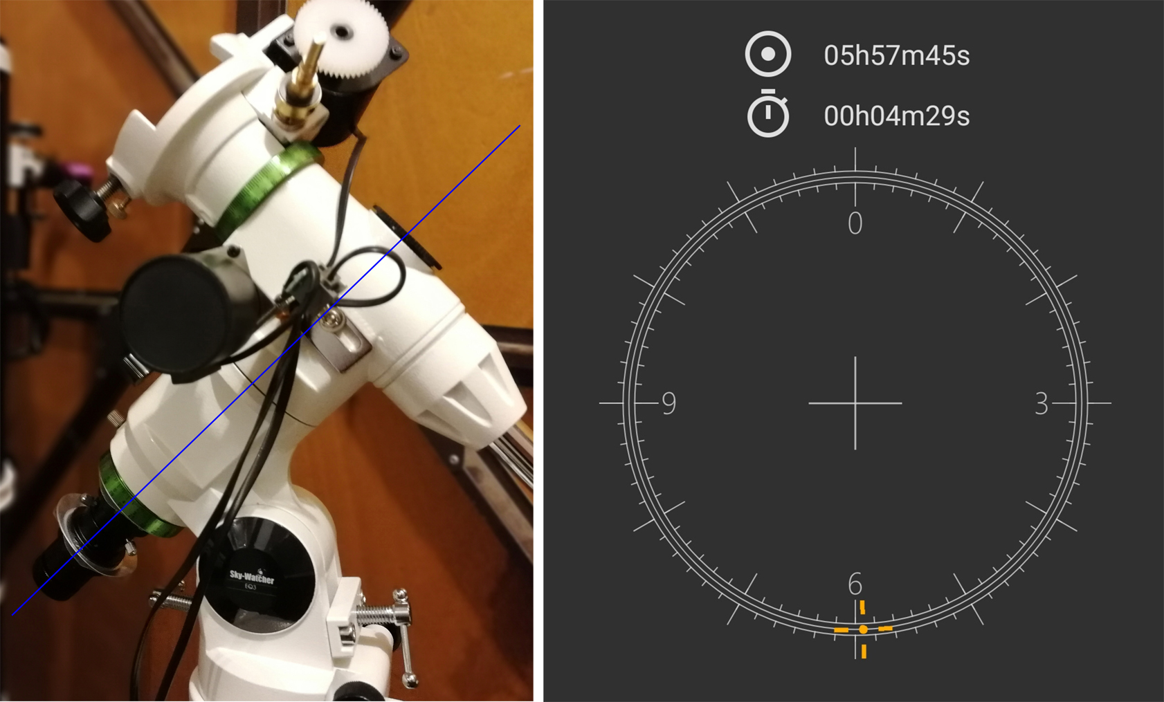
A key weakness intrinsic to my setup has been the alignment of the telescope’s equitorial mount: get it right and the target object stays centre-screen as the mount’s motors compensate for the rotation of the Earth; get it even slightly wrong and the target’s image will drift slowly away. The addition of a polarscope – a Christmas present – ought to have solved the problem. In essence this is a small telescope which fits directly to the mount and is designed to allow the system to be aligned using Polaris, the Pole Star. If the mount is set up correctly, then one can attach the telescope in the confident knowledge that a target object, once located, will be perfectly tracked thereafter. That’s the theory. In practice I had a false start because the polarscope wasn’t perfectly aligned with the axis of rotation of the mount: if the polarscope itself is misaligned then all the other steps in the process topple over. Using a point on a distant neighbour’s TV aerial as a daylight target I have overcome this particular stumbling block, I think. However, there next arises the need to position Polaris correctly in the polarscope’s field of view – it’s not at a point in the centre because Polaris is not precisely at 90º (i.e. above the Earth’s axis of rotation) but on one of a set of concentric circles at a position that varies with the time of day. I got this slightly wrong on the first outing so, although tracking was improved, I still couldn’t risk the longer exposure times necessary for fainter objects. I found an app for my ’phone which takes the work out of calculating Polaris’ position on the target circles so I am hopeful of being able to take another step forward next time the conditions are right.

The polarscope is shown above, fitted to be on the axis of rotation of my equitorial mount. (I've added a blue line to the image in order to highlight this.) Light from Polaris passes through a graticule within the small telescope and the mount’s alignment is fine-tuned to place Polaris on target – the appropriate position having been calculated by an app on my ’phone (see the screenshot on the right). Note that the angle of the polarscope/mount is 51.3º, this being my latitude. On an age-related note, I must add that the contortions I need to force upon my body in order to site Polaris through an eyepiece only 1-1.5 m above the ground and inclined at 51º are entirely non-trivial.

Locating objects remains a challenge unless they are bright or easily spotted in relation to readily identifiable stars/constellations nearby. There are two methods I hope to try in order to ease this problem. One is to place a known star in the centre of my field of view and then set the telescope mount’s celestial coordinates scales (its Right Ascension, RA, and declination, dec – akin to longitude and latitude respectively) to that star’s documented position. Thereafter, I ought to be able reliably to move the telescope to any given new object’s coordinates once I’ve looked them up. The second method I’m keen to try involves attaching my smartphone to the telescope using a suitable holder and undertaking an analogous process using one of the myriad of astronomy apps available. Thus, by sighting a known target in the telescope and then tweaking the alignment of my ’phone so that the corresponding object is displayed centre-screen, I ought then to be able to navigate to any other object using the app. Hopefully, this will take me to some of the fainter objects I might like to see such as a selection of nebulae and galaxies. This is all a work in progress, so we shall see.

_______________________________________

Extras, for those readers who just don’t know when to stop 😉

Useful Apps
I mentioned the image capture and processing software I use in my previous post and won’t cover them again here. What might be useful is a list of the apps I use; these are all for the Android operating system, but I’m sure there’ll be identical or similar apps available also for Apple/Windows ’phones:

• For general navigation around the night sky and to find the location of particular objects I mostly use Sky Map as I appreciate its simplicity of use; I also have SkySafari and SkEye installed and I use them also.
• The tool I have discovered as an aid to polar alignment is Polar Clock; PolarAligner can also be useful and I have it installed.
• By far the best tool I have found for identifying features on the Moon is LunarMap HD.
• Reliable forecasts for cloud cover are a real boon and I am grateful to my ex-colleague Dirk Froebrich, a professional astronomer, for pointing me towards Weather&Radar. This not only shows meteorological radar images in real time but also has the facility to run the clock forward: using the previous 90 minutes of radar data it displays the likely position of any clouds in user’s vicinity for the following 90 minutes. It’s not perfect but, in my experience, it’s pretty good.

Pixel counting
Large objects appear smaller if they are further away. This is as true in astronomy as it is in everyday life. Out of curiosity, I’ve taken a look back at the images I have managed to capture since beginning to try my hand at astrophotography and attempted to gauge their apparent size by counting the number of pixels from one side to the other. I say ‘attempted’ simply because there is a little uncertainty introduced by the optics: a point source of light is likely to show up in more than one of the camera detector’s pixels. At to that the effects of imperfect focusing, especially earlier on in my observations, and the ‘spread’ will become a more significant issue. This is a pretty universal issue, but it does mean that I need to make a ‘best guess’ estimate at the true extent of the object; the smaller the object appears, the larger the effect of any uncertainties.

Both the Sun and the Moon are huge in this respect: I cannot fit more than a fraction of their visible surface in my telescope/camera’s field of view. I do of course have the potential to image in relatively fine detail smaller areas on the surface – like individual lunar craters (down to about 15-20 km across) or the convection cell boundaries on the Sun – and this is a continuing source of delight.

In the same camp come many of the more easily located deep space objects, such as M42 (the star-forming nebula in Orion), M31 (Andromeda) or M45 (the Pleiades); each of them has an apparent size that exceeds by far the effective field of view of my telescope-camera setup. Perhaps counter-intuitively, magnification is not always the most valuable thing associated with a telescope – these deep space objects are a case in point. The key benefit of a telescope for objects such as these is its large aperture: it’s good at ‘gathering light’. Combine the large aperture with a long exposure time (more usually, a computer-managed stack of hundreds⸱⸱⸱thousands of individual exposures) and it becomes possible to reveal details and colours simply not visible otherwise. Whilst my setup is pretty good for viewing planets or individual stars it has too narrow a field of view for the more extensive objects. A larger chip than the 2 Mp one in my astro-camera would help, but I’d ideally also have a second, smaller telescope. It’s not going to happen; thankfully, I have a very long list of fascinating and beautiful objects still to capture for which my setup will do nicely.

Individual stars are at the other end of the scale. Mizar and Sirius both look to be in the region of two pixels in diameter, with Mizar probably appearing a shade smaller. Betelgeuse on the other hand, a red giant, steps this up to roughly three pixels across. (Creating purposefully unfocused images is actually a good way to reveal the differences in star colours.)

If now we turn to the planets in our Solar System the whole distance-apparent size phenomenon really begins to show up. For instance, when Mars was near its closest approach to the Earth during 2020 it appeared to be approximately 39 pixels across – meaning that some surface detail could be seen. This dropped to about half once the separation between us had increased again. Jupiter is almost three and a half times further away from the Sun as is Mars (779 M km and 228 M km respectively), but at about the same time as Mars appeared to have a diameter approaching 40 pixels Jupiter presented at a whopping 140 pixels across. Jupiter is really big. Even Saturn, further away still at 1,434 M km, appears as big as Mars: the planet itself measuring 37 pixels in diameter, with the rings taking this figure up to about 80 pixels. Similarly, Venus weighs in at 42 pixels across whereas the much larger but far, far more distant planet Uranus (2,871 M km from the Sun) shared its blue-green face across a circle of diameter 11 pixels only. If you would like a less casual approach to this question of apparent size I suggest the excellent article available here. Now, it is technically possible to increase the magnification of my telescope+camera from its current value of 48X by interposing a ‘Barlow lens’ between the telescope and the astro-camera. This is a diverging lens and it has the effect of increasing the effective focal length of the telescope, commonly by a factor of two. This would take my setup to 96X magnification. One day I shall try this – but it requires absolutely ideal observing conditions since that increased magnification will accentuate the effects of atmospheric turbulence and one might end up no better off overall. (The likelihood of such ideal conditions falling on a day when both the planet and I are available is not high in the UK.)